Source
import numpy as np
import matplotlib.pyplot as plt
plt.rcParams.update({
    "figure.figsize": (7, 3.6), "figure.dpi": 110,
    "axes.spines.top": False, "axes.spines.right": False,
    "axes.grid": True, "grid.alpha": 0.25, "font.size": 10,
})
rng = np.random.default_rng(7) # fixed seed so the text matches the plotsIn Section 3.2 the sensor models were simply given: “a plate’s ratio is about 0.10 ± 0.04”, and so on. Where do such numbers come from? In practice, an engineer puts real vessels through the machine, writes down what each one was (the label), and records what every sensor reported. The robot then learns its models from these labelled examples.
Learning brings new questions. How many examples are enough? What if some vessel types are rare? And how do we know whether the robot’s remaining mistakes come from too little data or from sensors that simply cannot tell certain vessels apart?
Source
vessels  = ["plate", "tumbler", "bowl", "cooking vessel", "other"]
short    = ["plate", "tumbler", "bowl", "cooking", "other"]
programs = ["quick rinse", "standard", "heavy degrease", "gentle"]
cost = np.array([[3, 1, 3, 12, 4],
                 [2, 2, 2,  8, 5],
                 [4, 4, 4,  3, 9],
                 [5, 4, 5, 10, 2]], dtype=float)
# ---- The TRUE world. The robot never sees these numbers; it only sees labelled examples. ----
true_prior = np.array([0.40, 0.25, 0.20, 0.10, 0.05])
true_a = (np.array([0.10, 1.30, 0.45, 0.40, 0.60]), np.array([0.04, 0.20, 0.10, 0.12, 0.35]))
true_w = (np.array([180, 90, 150, 900, 250.]),      np.array([40, 20, 40, 250, 150.]))
true_g = np.array([0.30, 0.05, 0.35, 0.90, 0.40])

def gauss(z, m, s):
    return np.exp(-0.5 * ((z - m) / s) ** 2) / (s * np.sqrt(2 * np.pi))

def collect(n):
    # Wash n labelled vessels on the test bench and record every sensor
    x = rng.choice(5, size=n, p=true_prior)
    ratio  = np.maximum(0.02, rng.normal(true_a[0][x], true_a[1][x]))
    weight = np.maximum(20.0, rng.normal(true_w[0][x], true_w[1][x]))
    greasy = (rng.random(n) < true_g[x]).astype(int)
    return x, ratio, weight, greasy
A labelled dataset
The engineer washes 300 vessels from the family’s kitchen, one at a time, and records the label and the three sensor readings for each. The first few rows of the log look like this:
x, ratio, weight, greasy = collect(300)
print(f"{'#':>3} | {'label':>14} | ratio | weight [g] | greasy")
for i in range(8):
    print(f"{i + 1:>3} | {vessels[x[i]]:>14} | {ratio[i]:5.2f} | {weight[i]:10.0f} | {'yes' if greasy[i] else 'no'}")
print("…")
print("vessels of each type:", dict(zip(short, np.bincount(x, minlength=5))))
# | label | ratio | weight [g] | greasy
1 | tumbler | 1.34 | 98 | no
2 | cooking vessel | 0.37 | 823 | yes
3 | bowl | 0.43 | 164 | yes
4 | plate | 0.10 | 140 | no
5 | plate | 0.16 | 114 | no
6 | cooking vessel | 0.47 | 1045 | yes
7 | plate | 0.10 | 178 | no
8 | bowl | 0.39 | 162 | no
…
vessels of each type: {'plate': np.int64(120), 'tumbler': np.int64(74), 'bowl': np.int64(61), 'cooking': np.int64(33), 'other': np.int64(12)}
Learning by counting and averaging
The prior. The simplest estimate of how often each type appears is its fraction in the data. If vessels of type appear among in total:
The grease sensor. If of the vessels of type came out greasy, the natural estimate is the fraction that did:
The camera and the scale. For a Gaussian model, the estimates are the sample mean and sample standard deviation of the readings for each type, exactly as for the tadka thermometer in Section 2.1.
These are called maximum-likelihood estimates: of all possible parameter values, they are the ones that make the observed data most probable. For counts and Gaussians, they turn out to be the everyday “fraction” and “average” we would have guessed anyway.
def fit(x, ratio, weight, greasy, alpha=1.0):
    K = 5
    counts = np.bincount(x, minlength=K).astype(float)
    prior = (counts + alpha) / (counts.sum() + K * alpha)
    a_m, a_s, w_m, w_s, g = (np.zeros(K) for _ in range(5))
    for k in range(K):
        m = x == k
        if m.sum() >= 2:
            a_m[k], a_s[k] = ratio[m].mean(), ratio[m].std(ddof=1)
            w_m[k], w_s[k] = weight[m].mean(), weight[m].std(ddof=1)
        else:  # too few examples: fall back to a vague model built from all the data
            a_m[k], a_s[k] = ratio.mean(), ratio.std()
            w_m[k], w_s[k] = weight.mean(), weight.std()
        a_s[k], w_s[k] = max(a_s[k], 0.02), max(w_s[k], 10.0)   # never trust a spread of almost zero
        g[k] = (greasy[m].sum() + alpha) / (m.sum() + 2 * alpha)
    return dict(prior=prior, a=(a_m, a_s), w=(w_m, w_s), g=g)

model = fit(x, ratio, weight, greasy)
print(f"{'type':>8} |  prior true/est  | ratio mean true/est | weight mean true/est | P(greasy) true/est")
for k in range(5):
    print(f"{short[k]:>8} |   {true_prior[k]:.2f} / {model['prior'][k]:.2f}   |"
          f"     {true_a[0][k]:.2f} / {model['a'][0][k]:.2f}     |"
          f"      {true_w[0][k]:4.0f} / {model['w'][0][k]:4.0f}     |   {true_g[k]:.2f} / {model['g'][k]:.2f}")
type | prior true/est | ratio mean true/est | weight mean true/est | P(greasy) true/est
plate | 0.40 / 0.40 | 0.10 / 0.10 | 180 / 175 | 0.30 / 0.34
tumbler | 0.25 / 0.25 | 1.30 / 1.26 | 90 / 90 | 0.05 / 0.08
bowl | 0.20 / 0.20 | 0.45 / 0.44 | 150 / 150 | 0.35 / 0.30
cooking | 0.10 / 0.11 | 0.40 / 0.38 | 900 / 977 | 0.90 / 0.86
other | 0.05 / 0.04 | 0.60 / 0.50 | 250 / 263 | 0.40 / 0.21
With 300 examples most estimates land close to the truth. The rare “other” type is the least accurate, because only about a dozen of the 300 vessels were “other”. Estimates are only as good as the number of examples behind them.
The zero-probability problem
Suppose the engineer is in a hurry and collects only 40 vessels. Among them are 10 tumblers, and by chance none of them came out greasy (greasy tumblers are uncommon, only 5%). The plain counting rule (2) then says
The robot now believes that a greasy tumbler is impossible. That sounds harmless until a tumbler of buttermilk arrives and the grease sensor fires. Watch what happens:
# A tumbler: tall (ratio 1.28), light (95 g), and the grease sensor fires
obs_ratio, obs_weight, obs_greasy = 1.28, 95.0, 1

def decide(p_greasy):
    p = true_prior * gauss(obs_ratio, *true_a) * gauss(obs_weight, *true_w)
    p = p * (p_greasy if obs_greasy else 1 - p_greasy)
    p = p / p.sum()
    return p, programs[int(np.argmin(cost @ p))]

for label, pg_tumbler in [("plain counting: 0/10", 0 / 10), ("Laplace smoothing: (0+1)/(10+2)", 1 / 12)]:
    pg = true_g.copy(); pg[1] = pg_tumbler
    p, prog = decide(pg)
    print(f"{label:>32}: P(tumbler) = {p[1]:.3f}, most likely = {short[int(np.argmax(p))]:>7}, programme = {prog}")
plain counting: 0/10: P(tumbler) = 0.000, most likely = other, programme = gentle
Laplace smoothing: (0+1)/(10+2): P(tumbler) = 0.993, most likely = tumbler, programme = quick rinse
With plain counting, a single zero wipes out the tumbler completely. The camera and scale both shout “tumbler”, but multiplying by zero overrules them, and the robot picks a different type and the wrong programme. One unlucky zero in the training data can silence every other sensor.
The fix is Laplace smoothing: before counting, pretend we saw each outcome a small number of extra times, (usually 1):
With , the tumbler estimate becomes : small, but not impossible. The camera and scale can now be heard, and the robot correctly runs a quick rinse. The same idea protects the prior and the Gaussian spreads, which is why fit above adds to the type counts and never allows a spread of almost zero.
How much data is enough? The learning curve
To see how performance grows with data, we train on datasets of increasing size and test each model on a large, separate set of vessels it has never seen. Testing on fresh data matters: a model tested on its own training data looks better than it really is. A plot of test cost against training size is called a learning curve.
def log_gauss(z, m, s):
    return -0.5 * ((z - m) / s) ** 2 - np.log(s * np.sqrt(2 * np.pi))

def average_cost(model, test):
    xt, rt, wt, gt = test
    # add log-probabilities instead of multiplying tiny numbers, so nothing underflows to zero
    logP = (np.log(model["prior"]) + log_gauss(rt[:, None], *model["a"]) + log_gauss(wt[:, None], *model["w"])
            + np.log(np.where(gt[:, None] == 1, model["g"], 1 - model["g"])))
    P = np.exp(logP - logP.max(axis=1, keepdims=True))
    P /= P.sum(axis=1, keepdims=True)
    action = np.argmin(P @ cost.T, axis=1)
    return cost[action, xt].mean(), P.argmax(axis=1)

test = collect(20000)
true_model = dict(prior=true_prior, a=true_a, w=true_w, g=true_g)
best_with_sensors = average_cost(true_model, test)[0]
oracle = cost[:, test[0]].min(axis=0).mean()

sizes = [10, 20, 40, 80, 160, 320, 640, 1280]
curve = [np.mean([average_cost(fit(*collect(n)), test)[0] for _ in range(15)]) for n in sizes]
for n, c in zip(sizes, curve):
    print(f"{n:>5} training vessels → average test cost {c:.3f}")
print(f"true sensor models → {best_with_sensors:.3f}   |   oracle → {oracle:.3f}")
10 training vessels → average test cost 2.691
20 training vessels → average test cost 2.496
40 training vessels → average test cost 2.136
80 training vessels → average test cost 2.033
160 training vessels → average test cost 1.975
320 training vessels → average test cost 1.969
640 training vessels → average test cost 1.964
1280 training vessels → average test cost 1.962
true sensor models → 1.959 | oracle → 1.865
plt.semilogx(sizes, curve, "o-", c="#1f3a5f", lw=2, label="learned models")
plt.axhline(best_with_sensors, c="#e07a3a", ls="--", label="true sensor models (limit of learning)")
plt.axhline(oracle, c="#2e8b57", ls="--", label="oracle (perfect sensing)")
plt.axhline(2.75, c="#9a4a16", ls=":", label="no sensors")
plt.xlabel("number of labelled training vessels"); plt.ylabel("average cost on new vessels")
plt.legend(fontsize=8); plt.title("Learning curve");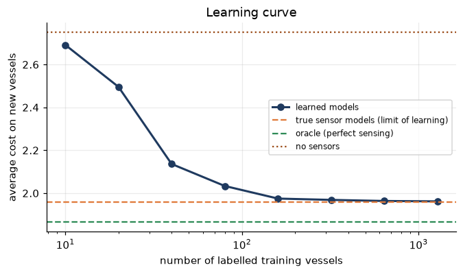
Figure 1:Learning curve for the vessel-washing robot. Test cost falls quickly as training data grows, then flattens at the level set by the sensors themselves (orange dashed line). The remaining gap to the oracle (green dashed line) cannot be closed with more data.
The curve tells a clear story:
Early on, data is precious. Going from 10 to 80 training vessels cuts the cost sharply. With very few examples, rare types have unreliable models, and the robot makes costly mistakes.
Then returns diminish. After a few hundred vessels the curve flattens against the orange line, the best these three sensors could ever do even with perfect models.
The final gap is not a data problem. The distance between the orange and green lines is caused by vessels the sensors genuinely cannot tell apart. A million more examples would not remove it.
Where the remaining mistakes are: the confusion matrix
A confusion matrix shows, for each true type (row), how often the robot predicted each type (column). The diagonal holds the correct answers, and everything off the diagonal is a mistake.
model500 = fit(*collect(500))
_, pred = average_cost(model500, test)
cm = np.zeros((5, 5))
for t, p in zip(test[0], pred):
    cm[t, p] += 1
cm /= cm.sum(axis=1, keepdims=True)
fig, ax = plt.subplots(figsize=(5.4, 4.4))
ax.imshow(cm, cmap="Blues", vmin=0, vmax=1); ax.grid(False)
ax.set_xticks(range(5), short, rotation=30); ax.set_yticks(range(5), short)
for i in range(5):
    for j in range(5):
        ax.text(j, i, f"{cm[i, j]:.2f}", ha="center", va="center", fontsize=8, color="white" if cm[i, j] > 0.5 else "black")
ax.set_xlabel("predicted type"); ax.set_ylabel("true type"); plt.tight_layout()
print("correct fraction for each true type:", dict(zip(short, np.round(np.diag(cm), 2))))
print("where 'other' vessels end up:", dict(zip(short, np.round(cm[4], 2))))
correct fraction for each true type: {'plate': np.float64(1.0), 'tumbler': np.float64(1.0), 'bowl': np.float64(0.98), 'cooking': np.float64(0.98), 'other': np.float64(0.53)}
where 'other' vessels end up: {'plate': np.float64(0.09), 'tumbler': np.float64(0.05), 'bowl': np.float64(0.24), 'cooking': np.float64(0.09), 'other': np.float64(0.53)}
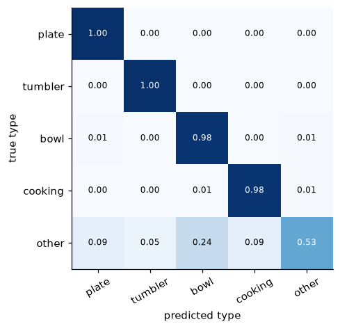
Figure 2:Confusion matrix of a model trained on 500 vessels and tested on 20 000 new ones. Rows are true types; columns are predictions; each row sums to 1. Nearly all mistakes involve the “other” type, whose shapes and weights overlap with everything else.
Plates, tumblers, bowls, and cooking vessels are recognised almost perfectly. The weak spot is “other”: the non-stick tawa, sieve, and glass jar have shapes and weights that overlap with ordinary vessels. Only about half are recognised; about a quarter are mistaken for bowls, and the rest are spread over the other types.
The mistakes are not equally serious. An “other” item mistaken for a bowl gets standard, which is merely too rough. One mistaken for a cooking vessel (about 9% of them here) gets heavy degrease, the one programme that ruins a non-stick coating. “Other” is exactly the type where a wrong programme can damage a vessel, so it deserves attention even though it is rare.
More data, or a better sensor?
The learning curve and the confusion matrix together answer the engineer’s most practical question.
| What you see | What it means | What to do |
|---|---|---|
| Test cost still falling steeply as data grows | the models are data-starved | collect more labelled examples |
| Test cost flat, near the limit of the true sensor models | the sensors cannot separate some types | add or improve a sensor |
| Mistakes concentrated in one type | that type needs its own clue | design a sensor aimed at that type |
For our robot, the curve is flat and the mistakes are concentrated in “other”. More data will not help. A sensor that recognises non-stick coatings and glass, for instance a small reflectance sensor that measures how shiny the surface is, would target exactly the remaining gap.
The chapter summary collects the ideas and exercises from all three sections.