2.1 Probability for Robots - Robots That Perceive

▶ Open this notebook in JupyterLab

import numpy as np
import matplotlib.pyplot as plt
plt.rcParams.update({
    "figure.figsize": (7, 3.6), "figure.dpi": 110,
    "axes.spines.top": False, "axes.spines.right": False,
    "axes.grid": True, "grid.alpha": 0.25, "font.size": 10,
})
rng = np.random.default_rng(42)  # fixed seed so the book text matches the plots

Robots are never certain. Probability is the language we use to say how uncertain they are, and to update that uncertainty as evidence arrives. This section covers the minimum needed for the rest of the book; Thrun et al., 2005 treats the subject in depth.

Discrete random variables¶

A discrete random variable $X$ takes values from a finite set. Its probability mass function assigns a probability to each value:

P(X = x) \ge 0, \qquad \sum_x P(X = x) = 1

(1)

For example, the type of the next vessel arriving at a washing station might follow this PMF:

categories = ["steel plate", "tumbler", "kadai", "tawa", "cooker lid"]
pmf = np.array([0.20, 0.30, 0.25, 0.20, 0.05])
assert np.isclose(pmf.sum(), 1)

samples = rng.choice(len(categories), size=500, p=pmf)
freq = np.bincount(samples, minlength=len(categories)) / len(samples)

xpos = np.arange(len(categories))
plt.bar(xpos - 0.2, pmf, 0.4, label="true PMF")
plt.bar(xpos + 0.2, freq, 0.4, label="frequency in 500 samples")
plt.xticks(xpos, categories); plt.ylabel("probability"); plt.legend(); plt.title("Sampling a categorical distribution");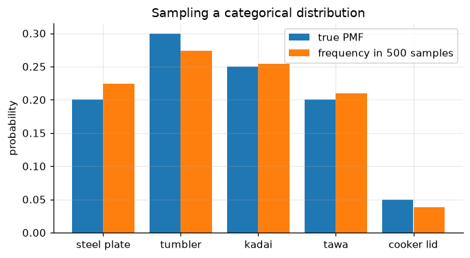

The law of large numbers¶

The sample frequencies approach the true probabilities as the number of samples grows. This is why simulation is a valid tool for reasoning about uncertainty:

N = 5000
draws = rng.choice(len(categories), size=N, p=pmf)
running = np.cumsum(draws == 2) / np.arange(1, N + 1)   # running frequency of "can"
plt.semilogx(np.arange(1, N + 1), running, label="running frequency of 'kadai'")
plt.axhline(pmf[2], c="k", ls="--", label="true probability 0.25")
plt.xlabel("number of samples"); plt.ylabel("estimate"); plt.legend(); plt.title("Law of large numbers");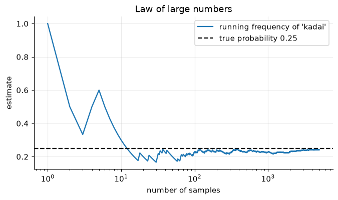

Continuous random variables and the Gaussian¶

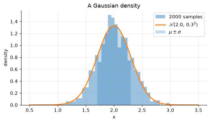
Positions, distances, and angles are continuous. We describe them with a probability density function $p(x)$ , whose integral over an interval gives a probability. The most important density in robotics is the Gaussian (normal) distribution:

\mathcal{N}(x;\,\mu,\sigma^2) = \frac{1}{\sqrt{2\pi\sigma^2}} \exp\!\left(-\frac{(x-\mu)^2}{2\sigma^2}\right)

(2)

It is fully described by its mean $\mu = \mathbb{E}[X]$ and variance $\sigma^2 = \mathbb{E}[(X-\mu)^2]$ . About 68% of the probability lies within $\mu \pm \sigma$ , and about 95% within $\mu \pm 2\sigma$ .

def gaussian(x, mu, sigma):
    return np.exp(-0.5 * ((x - mu) / sigma) ** 2) / np.sqrt(2 * np.pi * sigma ** 2)

mu, sigma = 2.0, 0.3
s = rng.normal(mu, sigma, 2000)
xs = np.linspace(0.5, 3.5, 400)
plt.hist(s, bins=40, density=True, alpha=0.45, label="2000 samples")
plt.plot(xs, gaussian(xs, mu, sigma), lw=2, label=r"$\mathcal{N}(2.0,\,0.3^2)$")
plt.fill_between(xs, gaussian(xs, mu, sigma), where=abs(xs - mu) < sigma, alpha=0.25, label=r"$\mu\pm\sigma$")
plt.xlabel("x"); plt.ylabel("density"); plt.legend(); plt.title("A Gaussian density")
print(f"sample mean {s.mean():.3f}, sample std {s.std():.3f}, fraction within 1σ: {np.mean(abs(s - mu) < sigma):.3f}")

sample mean 2.010, sample std 0.303, fraction within 1σ: 0.669

Joint and conditional probability¶

With two random variables we care about how they relate. The conditional probability of $A$ given $B$ is

P(A \mid B) = \frac{P(A, B)}{P(B)}

(3)

Rearranged, this is the product rule $P(A, B) = P(A \mid B)\,P(B)$ . Together with the sum rule $P(A) = \sum_b P(A, B=b)$ , it is all we need to derive Bayes’ rule in Section 2.3.