2.2 Sensors and Noise - Robots That Perceive

▶ Open this notebook in JupyterLab

import numpy as np
import matplotlib.pyplot as plt
plt.rcParams.update({
    "figure.figsize": (7, 3.6), "figure.dpi": 110,
    "axes.spines.top": False, "axes.spines.right": False,
    "axes.grid": True, "grid.alpha": 0.25, "font.size": 10,
})
rng = np.random.default_rng(42)  # fixed seed so the book text matches the plots

A sensor converts some physical property of the world into a number. That number depends on the state, but not perfectly. A sensor model captures this relationship as a conditional probability $p(z \mid x)$ : if the state were $x$ , how likely is reading $z$ ?

A range sensor¶

An ultrasonic range sensor measures distance to a wall. A common model assumes the reading equals the true distance plus Gaussian noise:

p(z \mid x) = \mathcal{N}(z;\, x,\, \sigma_z^2)

(1)

Real sensors also fail in less tidy ways, returning a maximum-range reading when the echo is lost or a random value from crosstalk. A standard trick is to model the sensor as a mixture of these effects Thrun et al., 2005:

true_dist, sigma_z, z_max = 2.0, 0.05, 5.0
w_hit, w_max, w_rand = 0.85, 0.08, 0.07

def sample_range(n):
    kind = rng.choice(3, size=n, p=[w_hit, w_max, w_rand])
    z = np.where(kind == 0, rng.normal(true_dist, sigma_z, n),
        np.where(kind == 1, z_max, rng.uniform(0, z_max, n)))
    return np.clip(z, 0, z_max)

z = sample_range(3000)
plt.hist(z, bins=120, density=True, alpha=0.7)
plt.xlabel("reading z [m]"); plt.ylabel("density"); plt.title("Simulated range readings of a wall 2 m away");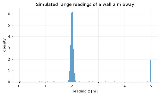

From sensor model to likelihood¶

The sensor model is a function of $z$ for a fixed $x$ . After a reading arrives, we fix $z$ and view the same expression as a function of $x$ . This is the likelihood $L(x) = p(z \mid x)$ . It is not a probability distribution over $x$ (it need not integrate to 1), but it tells us which states explain the reading well.

def p_range(z, x):
    hit = np.exp(-0.5 * ((z - x) / sigma_z) ** 2) / np.sqrt(2 * np.pi * sigma_z ** 2)
    rand = 1 / z_max
    return w_hit * hit + w_rand * rand      # (max-range spike omitted for z < z_max)

xs = np.linspace(0, 4, 800)
fig, ax = plt.subplots(1, 2, figsize=(9, 3.3))
zs = np.linspace(0, 4, 800)
ax[0].plot(zs, p_range(zs, 2.0)); ax[0].set_title("sensor model $p(z\\mid x=2)$"); ax[0].set_xlabel("z")
for z_obs in [1.2, 2.0, 3.1]:
    ax[1].plot(xs, p_range(z_obs, xs), label=f"z = {z_obs}")
ax[1].set_title("likelihood $L(x)=p(z\\mid x)$"); ax[1].set_xlabel("x"); ax[1].legend()
plt.tight_layout()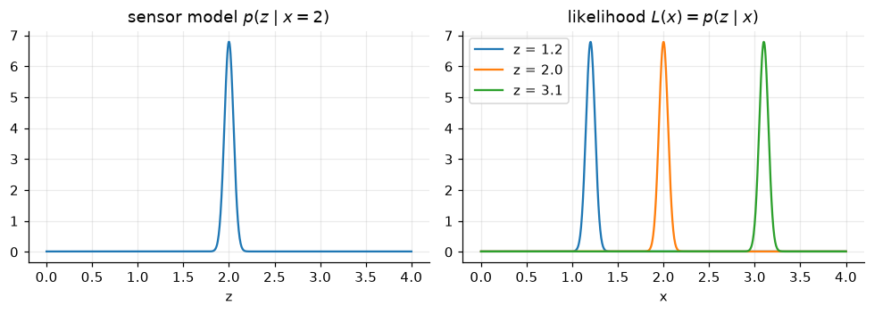

Binary sensors: false positives and negatives¶

Many sensors report only yes or no: is there a door here?, is the object metallic? Such a sensor is described by two numbers:

True-positive rate $P(z = 1 \mid x = 1)$ : how often it fires when the thing is present.
False-positive rate $P(z = 1 \mid x = 0)$ : how often it fires when the thing is absent.

The complements are the false-negative rate and the true-negative rate. A sensor with a 90% true-positive rate sounds good, but if the thing it detects is rare, most of its detections can still be wrong. Section 2.3 shows why.

p_tp, p_fp = 0.9, 0.1
for prior in [0.5, 0.1, 0.01]:
    p_fire = p_tp * prior + p_fp * (1 - prior)
    p_present_given_fire = p_tp * prior / p_fire
    print(f"prior {prior:5.2f} -> P(present | sensor fires) = {p_present_given_fire:.3f}")

prior  0.50 -> P(present | sensor fires) = 0.900
prior  0.10 -> P(present | sensor fires) = 0.500
prior  0.01 -> P(present | sensor fires) = 0.083