2.3 Bayesian Inference - Robots That Perceive

▶ Open this notebook in JupyterLab

import numpy as np
import matplotlib.pyplot as plt
plt.rcParams.update({
    "figure.figsize": (7, 3.6), "figure.dpi": 110,
    "axes.spines.top": False, "axes.spines.right": False,
    "axes.grid": True, "grid.alpha": 0.25, "font.size": 10,
})
rng = np.random.default_rng(42)  # fixed seed so the book text matches the plots

Perception is inference: given measurements, what is the state? Bayes’ rule answers this by combining what we believed beforehand with how well each state explains the evidence.

Bayes’ rule¶

Applying the product rule both ways, $P(x, z) = P(z \mid x)P(x) = P(x \mid z)P(z)$ , and solving for the quantity we want gives

\underbrace{P(x \mid z)}_{\text{posterior}} = \frac{\overbrace{P(z \mid x)}^{\text{likelihood}}\;\overbrace{P(x)}^{\text{prior}}}{\underbrace{P(z)}_{\text{evidence}}} \;\propto\; P(z \mid x)\,P(x)

(1)

The evidence $P(z) = \sum_x P(z\mid x)P(x)$ does not depend on $x$ , so in practice we multiply prior by likelihood and then normalize so the result sums to one.

Where am I in the corridor?¶

A robot is somewhere in a corridor divided into 20 cells. Some cells have doors. Its door sensor has a true-positive rate of 0.85 and a false-positive rate of 0.15. The robot does not move in this example; it simply takes readings while standing in place.

doors = np.zeros(20, dtype=int); doors[[2, 5, 11, 16]] = 1
p_tp, p_fp = 0.85, 0.15

def likelihood(z):
    # P(z | x) for every cell x at once
    p_fire = np.where(doors == 1, p_tp, p_fp)
    return p_fire if z == 1 else 1 - p_fire

def bayes_update(prior, z):
    post = likelihood(z) * prior
    return post / post.sum()

true_cell = 11
prior = np.full(20, 1 / 20)
beliefs = [prior]
for _ in range(4):
    z = int(rng.random() < (p_tp if doors[true_cell] else p_fp))
    beliefs.append(bayes_update(beliefs[-1], z))

fig, axes = plt.subplots(len(beliefs), 1, figsize=(7, 6), sharex=True)
for i, (ax, b) in enumerate(zip(axes, beliefs)):
    ax.bar(range(20), b, color=np.where(doors, "tab:orange", "tab:blue"))
    ax.axvline(true_cell, c="k", ls=":", lw=1)
    ax.set_ylabel("prior" if i == 0 else f"after z{i}")
axes[-1].set_xlabel("cell (orange = door)"); fig.suptitle("Repeated Bayesian updates"); plt.tight_layout()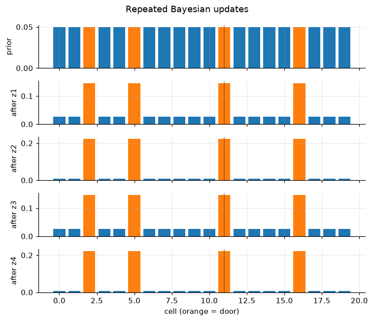

Each “door seen” reading shifts probability toward the door cells. Because the robot is not moving, however, it can never tell which door it is standing at, and the belief stays split across four peaks. Resolving this ambiguity requires motion plus sensing, which is the Bayes filter we build in Chapter 6.

MAP and posterior mean¶

A belief is a whole distribution, but we often need a single answer. Two common choices:

\hat{x}_{\text{MAP}} = \arg\max_x P(x \mid z), \qquad \hat{x}_{\text{MMSE}} = \mathbb{E}[x \mid z] = \sum_x x\,P(x \mid z)

(2)

With a multimodal belief like the one above, the posterior mean can land between doors, where the robot certainly is not. That is a warning that summarizing a belief by one number throws information away.

post = beliefs[-1]
print("MAP cell:", int(np.argmax(post)), "| posterior mean:", round(float(np.sum(np.arange(20) * post)), 2))

MAP cell: 2 | posterior mean: 8.64

Continuous Bayes: fusing two Gaussians¶

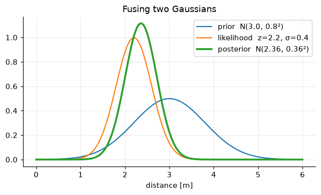
When both prior and likelihood are Gaussian, the posterior is also Gaussian, and the update has a closed form. For a prior $\mathcal{N}(\mu_0, \sigma_0^2)$ and a measurement $z$ with noise $\sigma_z^2$ :

\mu_1 = \frac{\sigma_z^2\,\mu_0 + \sigma_0^2\,z}{\sigma_0^2 + \sigma_z^2}, \qquad \sigma_1^2 = \frac{\sigma_0^2\,\sigma_z^2}{\sigma_0^2 + \sigma_z^2}

(3)

The posterior mean is a weighted average that trusts the less noisy source more, and the posterior variance is always smaller than either input. This one equation is the heart of the Kalman filter in Chapter 7.

mu0, s0 = 3.0, 0.8      # prior belief about distance
z, sz   = 2.2, 0.4      # measurement and its noise
mu1 = (sz**2 * mu0 + s0**2 * z) / (s0**2 + sz**2)
s1  = np.sqrt(s0**2 * sz**2 / (s0**2 + sz**2))
xs = np.linspace(0, 6, 500)
g = lambda x, m, s: np.exp(-0.5 * ((x - m) / s) ** 2) / (s * np.sqrt(2 * np.pi))
plt.plot(xs, g(xs, mu0, s0), label=f"prior  N({mu0}, {s0}²)")
plt.plot(xs, g(xs, z, sz), label=f"likelihood  z={z}, σ={sz}")
plt.plot(xs, g(xs, mu1, s1), lw=2.5, label=f"posterior  N({mu1:.2f}, {s1:.2f}²)")
plt.xlabel("distance [m]"); plt.legend(); plt.title("Fusing two Gaussians");