Source
import numpy as np
import matplotlib.pyplot as plt
plt.rcParams.update({
    "figure.figsize": (7, 3.6), "figure.dpi": 110,
    "axes.spines.top": False, "axes.spines.right": False,
    "axes.grid": True, "grid.alpha": 0.25, "font.size": 10,
})
rng = np.random.default_rng(7) # fixed seed so the text matches the plotsLook around an Indian home on a busy morning. The mixer-grinder runs for as long as you hold the switch. The washing machine works through a fixed programme. The water-tank float switch cuts the motor when the tank is full. All of these are automatic, but most people would not call them robots.
Now imagine a mop that notices it has reached the edge of the rug and turns away, or a drone that holds its height steady while a gust of wind pushes it down. These machines do something the mixer-grinder cannot. They observe their surroundings, decide what to do based on what they observe, and act on that decision, again and again.
That is the working definition used throughout this book:
A robot is a machine that senses its environment, decides what to do using what it sensed, and acts on the physical world, in a continuing loop.
Robot or not?
The definition gives us three questions to ask about any machine: does it sense, does it decide, and does it act physically? Here are some familiar devices checked against it:
| Device | Senses? | Decides from what it senses? | Acts physically? | A robot? |
|---|---|---|---|---|
| Mixer-grinder | no | no (fixed speed and time) | yes | no |
| Water-tank float switch | yes (water level) | a single on/off rule | yes (motor switch) | a borderline case |
| Automatic washing machine | yes (load weight, water level) | chooses water amount and time | yes | a simple robot |
| Floor-mopping robot | yes (bump, cliff, and range sensors) | plans where to clean next | yes | yes |
| Delivery drone | yes (GPS, camera, inertial sensors) | plans a route and holds a hover | yes | yes |
Robots sit on a spectrum. What moves a machine along it is how much its behavior depends on what it perceives, and how rich the decisions it makes are.
The sense–think–act loop
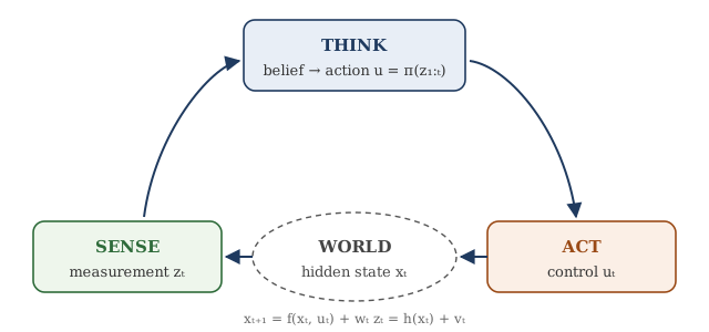
Figure 1:The sense–think–act loop. The world has a true state that the robot cannot observe directly. It receives measurements , updates what it believes, chooses an action , and the world changes in response.
Every robot in this book fits Figure 1. Three quantities appear again and again:
| Symbol | Name | Vessel-washing robot | Cooking arm | Delivery drone |
|---|---|---|---|---|
| state | type of vessel in the sink | joint angles of the arm | position, velocity, and tilt | |
| measurement | camera image, weight | joint encoder readings | GPS fix, barometer, gyroscope | |
| action | which wash programme to run | motor torques | four rotor speeds |
The robot’s decision rule is called a policy, written . In general it may use every measurement received so far:
Much of this book is about designing good policies of the form (1). A good policy usually works in two stages. First it estimates the state from the measurements, which is perception. Then it chooses an action given that estimate, which is reasoning and control.
A first robot: tempering oil for a tadka
Our first example is a small job for a kitchen robot: heating oil in a kadai to about 180 °C for a tadka, the moment when mustard seeds crackle but the oil does not smoke. The robot controls an induction cooktop and reads a thermometer probe dipped in the oil.
We model the oil and kadai together as one body with temperature (in °C). The heater delivers power (in watts), and heat leaks to the kitchen air at a rate proportional to how much hotter the oil is than the room:
Here is the heat capacity of oil and vessel (joules per °C), and describes the heat loss (watts per °C). The thermometer is noisy, so the robot measures , where is random noise.
We compare two strategies:
Open loop. Use the model to calculate in advance how long to run at full power, then switch to the steady power that should hold 180 °C. The thermometer is never consulted.
Closed loop. At every step, read the thermometer and set the power in proportion to the temperature error: , limited to what the cooktop can deliver.
Real kitchens do not follow the plan. In this simulation the cook poured in 30% more oil than the recipe assumed, and at s a handful of cold curry leaves and chopped onion drops the temperature.
# ---- Physical setup (change these and re-run) ---------------------------------
T_room, T_target = 30.0, 180.0      # °C
C_planned = 1700.0                  # heat capacity the plan assumes [J/°C]
C_actual  = 1.3 * C_planned         # the cook used 30% more oil
k_loss    = 8.0                     # heat loss to the room [W/°C]
P_max     = 2000.0                  # induction cooktop limit [W]
sensor_sd = 2.0                     # thermometer noise [°C]
t_add, drop = 150.0, 35.0           # time [s] and size [°C] of the ingredient drop
dt, T_end = 0.5, 400.0
# ---------------------------------------------------------------------------------
steps = int(T_end / dt)
time = np.arange(steps) * dt

def simulate(policy):
    T, temps, powers = T_room, [], []
    for i in range(steps):
        z = T + rng.normal(0, sensor_sd)            # sense
        P = float(np.clip(policy(time[i], z), 0, P_max))   # think
        T += dt * (P - k_loss * (T - T_room)) / C_actual   # act: the world responds
        if abs(time[i] - t_add) < dt / 2:
            T -= drop                                # ingredients go in
        temps.append(T); powers.append(P)
    return np.array(temps), np.array(powers)

# Open loop: full power for the time the (wrong) model says is needed, then a holding power
P_hold = k_loss * (T_target - T_room)
t_full = -C_planned / k_loss * np.log(1 - k_loss * (T_target - T_room) / P_max)
open_loop = lambda t, z: P_max if t < t_full else P_hold

# Closed loop: proportional feedback on the measured temperature
K_p = 300.0                                          # watts per °C of error
closed_loop = lambda t, z: K_p * (T_target - z)

T_open, P_open = simulate(open_loop)
T_closed, P_closed = simulate(closed_loop)
print(f"planned full-power time: {t_full:.0f} s")
planned full-power time: 195 s
fig, ax = plt.subplots(1, 2, figsize=(11, 3.6))
ax[0].plot(time, T_open, c="tab:orange", lw=2, label="open loop (timer)")
ax[0].plot(time, T_closed, c="tab:blue", lw=2, label="closed loop (thermometer)")
ax[0].axhline(T_target, c="k", ls="--", lw=1, label="target 180 °C")
ax[0].axvline(t_add, c="gray", ls=":", lw=1); ax[0].text(t_add + 4, 60, "ingredients\nadded", fontsize=8, color="gray")
ax[0].set_xlabel("time [s]"); ax[0].set_ylabel("oil temperature [°C]"); ax[0].legend(fontsize=8)
ax[1].plot(time, P_open, c="tab:orange", label="open loop")
ax[1].plot(time, P_closed, c="tab:blue", alpha=0.8, label="closed loop")
ax[1].set_xlabel("time [s]"); ax[1].set_ylabel("heater power [W]"); ax[1].legend(fontsize=8)
plt.tight_layout()
print(f"temperature at the end — open loop: {T_open[-1]:.0f} °C, closed loop: {T_closed[-1]:.0f} °C")
temperature at the end — open loop: 155 °C, closed loop: 176 °C
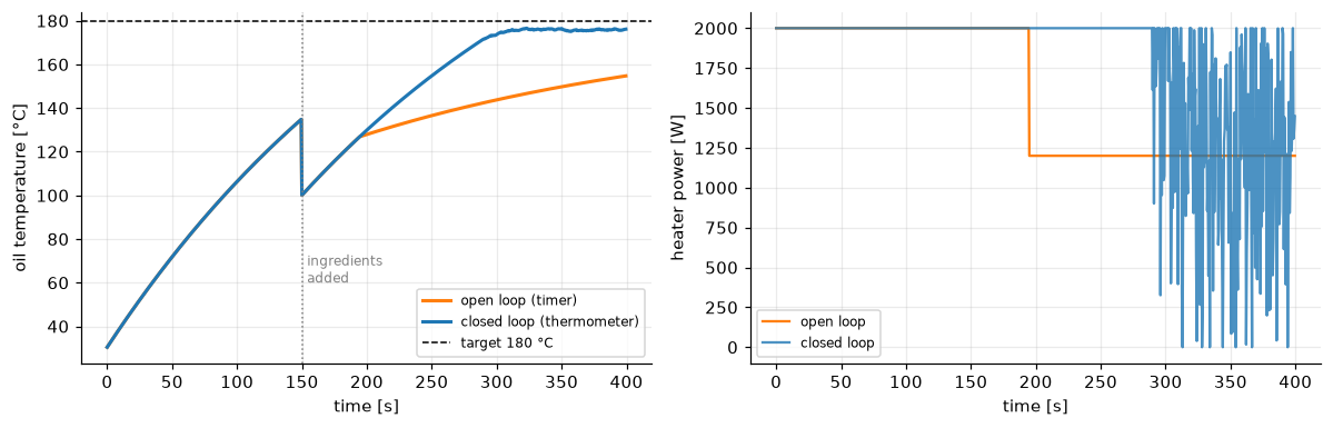
Figure 2:Heating oil for a tadka. The open-loop plan (orange) never reaches the target because there is more oil than it assumed, and it cannot recover from the drop when ingredients are added. The feedback controller (blue) settles a few degrees below 180 °C and recovers from the drop within seconds.
Three things in Figure 2 are worth noticing.
Feedback absorbs surprises. The closed-loop robot never knew there was extra oil or when the onions went in. It simply kept measuring and correcting.
The controller slows down by itself. Far from the target it runs at full power; close to the target the power falls. Nobody programmed “slow down near 180 °C”. It follows from making power proportional to the error.
It settles slightly below the target. To hold 180 °C the heater must supply about 1200 W, and a proportional controller only produces power when there is an error. The settled error is therefore about °C. Chapter 8 removes this kind of offset with integral action.
The jagged power curve shows the robot reacting to thermometer noise. Chapter 2 shows how to reason about noisy measurements so a robot reacts to what is real rather than to noise.
What makes robotics hard
The loop in Figure 1 looks simple, but each arrow hides a real difficulty. Each one is the subject of later chapters:
Uncertainty. Sensors are noisy and motors are imperfect, so the robot never knows exactly. We handle this with probability in Chapter 2.
Recognition. Turning raw sensor data into useful facts, such as “this is a greasy kadai, not a steel tumbler”, is its own problem (Chapter 3).
Geometry. A cooking arm has to know where its ladle is from its joint angles, and which angles will put the ladle in the pot (Chapter 4).
Maps and planning. A mopping robot must know which tiles it has cleaned, and a delivery robot must find a route through an apartment complex (Chapters 5 and 6).
Dynamics and other agents. Vehicles and drones obey Newton’s laws and share the road and sky with people who do not follow our plans (Chapters 7 and 8).
General introductions to the field include Siegwart et al., 2011, Lynch & Park, 2017, and Corke, 2017.
- Siegwart, R., Nourbakhsh, I. R., & Scaramuzza, D. (2011). Introduction to Autonomous Mobile Robots (2nd ed.). MIT Press.
- Lynch, K. M., & Park, F. C. (2017). Modern Robotics: Mechanics, Planning, and Control. Cambridge University Press.
- Corke, P. (2017). Robotics, Vision and Control: Fundamental Algorithms in MATLAB (2nd ed.). Springer.