1.2 State, Actions, and Models - Robots That Perceive

▶ Open this notebook in JupyterLab

import numpy as np
import matplotlib.pyplot as plt
plt.rcParams.update({
    "figure.figsize": (7, 3.6), "figure.dpi": 110,
    "axes.spines.top": False, "axes.spines.right": False,
    "axes.grid": True, "grid.alpha": 0.25, "font.size": 10,
})
rng = np.random.default_rng(7)  # fixed seed so the text matches the plots

Before a robot can reason about the world, we have to decide what it reasons about. This choice, called the state representation, is one of the most important modeling decisions in robotics. A good state contains just enough information to predict what happens next when the robot acts, and nothing more.

Choosing a state¶

Robot	A sensible state	Type
Vessel-washing robot	which kind of vessel is in the sink	discrete (one of a few types)
Mopping robot on a tiled floor	which tile it is on	discrete (grid cells)
Cooking arm	angle of each joint	continuous (a vector of angles)
Delivery robot in an apartment complex	position $(p_x, p_y)$ and heading $\theta$	continuous
Delivery drone	position, velocity, and orientation in 3D	continuous

A discrete state takes one of finitely many values. A continuous state is a vector of real numbers. The same robot can often be modeled either way: a mopping robot’s position is really continuous, but thinking in whole tiles makes planning much simpler.

Two models describe every robot¶

A motion model says how the state changes when the robot acts, and a measurement model says what the sensors report in a given state:

\text{motion model:}\qquad x_{t+1} = f(x_t, u_t) + w_t

(1)

\text{measurement model:}\qquad z_t = h(x_t) + v_t

(2)

The terms $w_t$ and $v_t$ are noise. $w_t$ captures the fact that the world does not do exactly what we command (wheels slip, wind blows), and $v_t$ captures sensor error. For discrete states we express the same ideas as conditional probabilities, $P(x_{t+1} \mid x_t, u_t)$ and $P(z_t \mid x_t)$ .

A discrete motion model: mopping a wet balcony¶

A mopping robot cleans a narrow balcony six tiles long, moving one tile at a time from tile 0 toward the wall at tile 5. The floor is wet, so its wheels are unreliable. When it commands “forward one tile”:

it moves one tile with probability 0.70,
it slips and stays where it is with probability 0.20,
it skids forward two tiles with probability 0.10.

At the wall it cannot go further. We collect these probabilities in a transition matrix $T$ , where entry $T_{ij} = P(x_{t+1} = j \mid x_t = i)$ . Each row is a probability distribution, so it sums to 1.

n_tiles = 6
p_move, p_stay, p_skid = 0.70, 0.20, 0.10
T = np.zeros((n_tiles, n_tiles))
for i in range(n_tiles):
    T[i, i] += p_stay
    T[i, min(i + 1, n_tiles - 1)] += p_move
    T[i, min(i + 2, n_tiles - 1)] += p_skid
print(np.round(T, 2))
print("rows sum to 1:", np.allclose(T.sum(axis=1), 1))

[[0.2 0.7 0.1 0.  0.  0. ]
 [0.  0.2 0.7 0.1 0.  0. ]
 [0.  0.  0.2 0.7 0.1 0. ]
 [0.  0.  0.  0.2 0.7 0.1]
 [0.  0.  0.  0.  0.2 0.8]
 [0.  0.  0.  0.  0.  1. ]]
rows sum to 1: True

If the robot starts certain that it is on tile 0 and commands “forward” several times, what should it believe about where it is? The probability of being on tile $j$ after one more step adds up all the ways of getting there:

P(x_{t+1} = j) = \sum_i P(x_t = i)\;T_{ij}

(3)

In matrix form this is a row vector times a matrix, $p_{t+1} = p_t\,T$ .

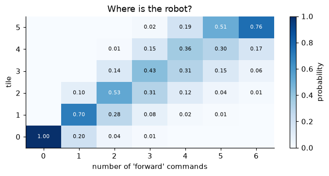
<Figure size 825x352 with 2 Axes> — Figure 1:Belief about the mopping robot’s tile after each “forward” command on a wet floor. Without sensing, the belief spreads over several tiles, and only the wall at tile 5 eventually concentrates it again.

After three commands the robot “should” be on tile 3, but it is actually there with only about 40% probability. Without a sensor that can tell tiles apart, the robot has no way to shrink this uncertainty until it reaches the wall. Mapping and localization in Chapters 5 and 6 are about exactly this problem.

A measurement model: ranging to a gate¶

A delivery robot measures its distance to an apartment gate with an ultrasonic range sensor. Real sensors of this kind become less precise with distance, so we model the noise standard deviation as growing with range:

z = d + v, \qquad v \sim \mathcal{N}\big(0,\ \sigma(d)^2\big), \qquad \sigma(d) = 0.02 + 0.03\,d \ \text{metres}

(4)

The notation $v \sim \mathcal{N}(0, \sigma^2)$ means “ $v$ is drawn from a Gaussian (bell-curve) distribution with mean 0 and standard deviation $\sigma$ ”. Section 2.1 explains it in detail. The sensor also reports only whole centimetres, and it cannot see beyond 4 m.

def ultrasonic(d, n=1):
    sigma = 0.02 + 0.03 * d
    z = d + rng.normal(0, sigma, n)
    z = np.round(z, 2)                    # whole centimetres
    return np.where(d > 4.0, np.nan, z)   # nothing beyond 4 m

d_true = np.repeat(np.linspace(0.2, 4.5, 60), 15)
z = np.array([ultrasonic(d)[0] for d in d_true])
ds = np.linspace(0.2, 4.0, 100)
plt.scatter(d_true, z, s=4, alpha=0.4, label="readings")
plt.plot(ds, ds, "k", lw=1, label="perfect sensor")
plt.fill_between(ds, ds - 2 * (0.02 + 0.03 * ds), ds + 2 * (0.02 + 0.03 * ds), alpha=0.2, label="±2σ band")
plt.axvline(4.0, c="r", ls=":", label="maximum range")
plt.xlabel("true distance to gate d [m]"); plt.ylabel("reading z [m]"); plt.legend(fontsize=8)
plt.title("Measurement model of an ultrasonic sensor");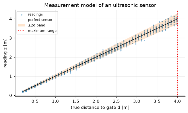

A measurement model like (4) tells us how far to trust each reading. A reading of 0.5 m can be trusted to within a few centimetres; a reading of 3.5 m could easily be 20 cm off. Beyond 4 m the sensor returns nothing at all, which is itself information: the gate is probably more than 4 m away.

A continuous motion model: the delivery robot drives¶

Now let the delivery robot drive along a path in the apartment complex. Its state is its position and heading $(p_x, p_y, \theta)$ . Each second it is commanded to drive forward at speed $v$ while turning at rate $\omega$ , and both are disturbed by noise from uneven paving:

\begin{aligned} \theta_{t+1} &= \theta_t + (\omega + w_\omega)\,\Delta t \\ p_{x,t+1} &= p_{x,t} + (v + w_v)\cos\theta_t\,\Delta t \\ p_{y,t+1} &= p_{y,t} + (v + w_v)\sin\theta_t\,\Delta t \end{aligned}

(5)

We cannot predict one exact future, but we can sample many possible futures and look at where they end up.

n_futures, dt = 300, 1.0
# Plan: 12 s straight, then a gentle left turn for 10 s, then straight for 6 s
plan = [(1.0, 0.0)] * 12 + [(1.0, np.pi / 2 / 10)] * 10 + [(1.0, 0.0)] * 6
sd_v, sd_w = 0.05, 0.03                 # noise on speed [m/s] and turn rate [rad/s]

state = np.zeros((n_futures, 3))        # columns: px, py, theta
paths = [state.copy()]
for v, w in plan:
    th = state[:, 2]
    vn = v + rng.normal(0, sd_v, n_futures)
    state[:, 0] += vn * np.cos(th) * dt
    state[:, 1] += vn * np.sin(th) * dt
    state[:, 2] += (w + rng.normal(0, sd_w, n_futures)) * dt
    paths.append(state.copy())
paths = np.array(paths)                 # (time, future, 3)

for k in range(60):
    plt.plot(paths[:, k, 0], paths[:, k, 1], c="tab:blue", lw=0.5, alpha=0.4)
for t, c in [(12, "tab:green"), (22, "tab:orange"), (28, "tab:red")]:
    plt.scatter(paths[t, :, 0], paths[t, :, 1], s=4, c=c, label=f"after {t} s")
plt.axis("equal"); plt.xlabel("$p_x$ [m]"); plt.ylabel("$p_y$ [m]"); plt.legend(fontsize=8)
plt.title("300 possible futures of the same plan");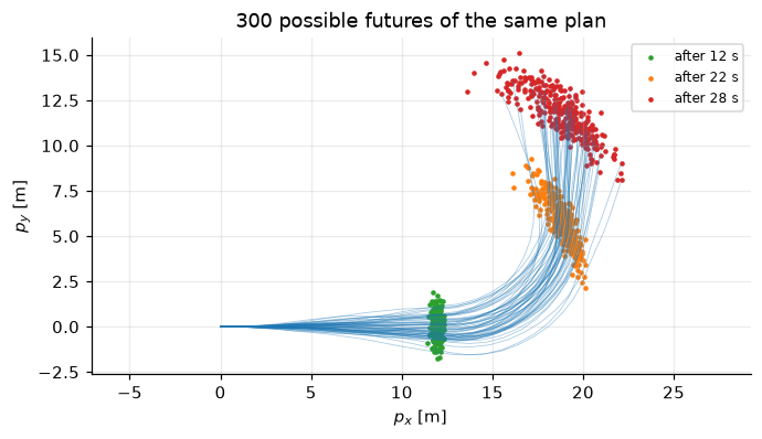

The clouds of possible positions grow as the robot drives. They also bend: small errors in heading turn into large sideways errors after a long straight run, so the cloud stretches across the direction of travel rather than along it. This shape is typical of wheeled robots, and it is why a delivery robot needs to keep correcting its estimate with landmarks and GPS.